AI has become the default answer to almost every question and being used as buzz word. So we tested seven machine-learning models through the same tests on two very different payments problems. The winner changed completely depending on the problem.
AI models now sit behind fraud screening, approval optimisation, reporting and much more. The temptation is to pick one powerful model and apply it everywhere.
Based on what we are seeing in our own platform, that approach leaves real performance on the table. When we benchmarked the most widely used model side by side, the best choice for one problem was close to the worst for another.
This matters for every merchant, PSP and acquirer investing in intelligent payments. The question is no longer whether to use machine learning, but which kind of model fits the shape of the problem in front of you.
What did we test?
We chose two problems that represent the two most common types of machine-learning task in payments.
The first is real-time classification: scoring each individual event as it happens and choosing the best of several options.
The second is intraday time-series forecasting: predicting where an aggregate measure will finish by the end of the day, updated as the day unfolds.
We ran seven approaches through both: four gradient-boosted tree models (LightGBM, XGBoost, CatBoost and HistGradientBoosting), a random forest, a simple linear model and a no-frills baseline built on historical averages.
Every model saw the same data and was judged only on periods it had never seen, the way it would be used in production.
| Type 1: real-time classification | Type 2: intraday time-series forecasting | |
| Task shape | Score each event and pick the best of several options | Forecast an aggregate total from the day’s partial data |
| Model output | Probability of a positive outcome for each option | End-of-day point forecast, refreshed hourly |
| Test design | 3 unseen days, ~2,930 events replayed | 30 unseen days, hourly forecasts, weekly retraining |
| Success measure | Uplift in positive-outcome rate vs current logic (pts) | Error reduction vs naive run-rate (%) |
| Also measured | Weakest day, calibration, latency, model size | Error by time of day, worst day, bias |
Type 1, real-time classification: boosted trees lead
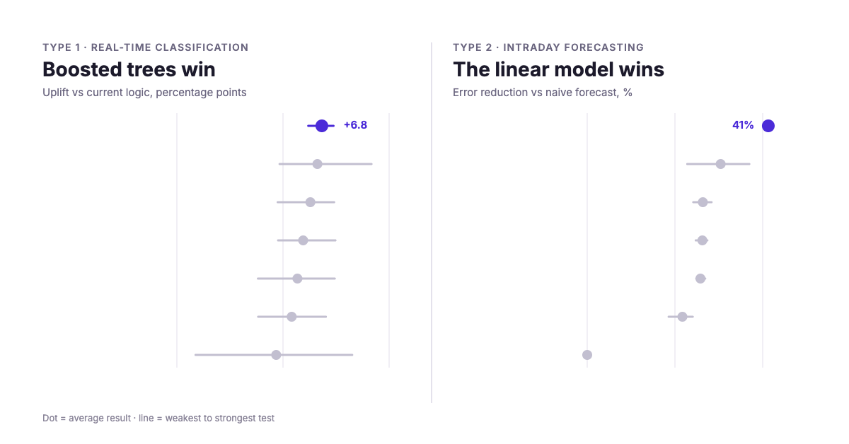
LightGBM came out on top On the classification task, . In replay testing across three separate days, it improved the positive-outcome rate by 6.8 percentage points over the existing logic, roughly 200 additional positive outcomes for every 3,000 events scored.
What stood out was consistency. Its weakest day still delivered a 6.2 point uplift, while every other model had at least one day that dipped below 5 points. The historical-average baseline looked respectable on average but dropped to under 1 point on a bad day.
Speed counts here too, because this kind of decision is made in real time. LightGBM scored every option in well under a millisecond. The random forest came close on accuracy but was 35 times slower and 22 times larger, which rules it out for real-time use. The linear model ranked options sensibly, but its probabilities were poorly calibrated, so any threshold or explanation built on them would be off.
| Model | Avg uplift (pts) | Weakest day (pts) | Calibration error (pts) | p99 latency (ms) | Model size (MB) |
| LightGBM | +6.83 | +6.19 | 1.8 | 0.67 | 0.6 |
| Random forest | +6.62 | +4.84 | 1.6 | 23.48 | 13.8 |
| HistGradientBoosting | +6.29 | +4.75 | 1.6 | 7.76 | 0.8 |
| XGBoost | +5.95 | +4.77 | 1.9 | 1.45 | 1.2 |
| Linear (logistic regression) | +5.68 | +3.82 | 7.7 | 1.61 | <0.1 |
| CatBoost | +5.41 | +3.83 | 1.7 | 0.58 | 1.7 |
| Historical-average baseline | +4.68 | +0.88 | 2.2 | ~0 | ~0 |
Uplift is measured against the existing decision logic in offline replay. Latency covers scoring up to eight options per event. Lower calibration error is better.
Type 2, intraday forecasting: the simple model wins
On forecasting, the result flipped. A regularised linear model cut forecast error by 41% compared with a naive run-rate projection. The tree-based models, LightGBM included, managed between 22% and 30%.
The linear model won on all three series we forecast. Its advantage was largest early and mid-day, exactly when a reliable forecast is most useful for acting before the day is lost. By late day, every model converged, because most of the answer is already in.
Even a carefully tuned tree-based forecaster did no better than an off-the-shelf one. More tuning was not the answer; a different kind of model was.
| Model | Error reduction vs naive (%) | Error, early day (%) | Error, mid-day (%) | Error, late day (%) | Worst-day error (%) |
| Linear (ridge regression) | 41.3 | 10.1 | 7.4 | 3.8 | 18.4 |
| CatBoost | 30.4 | 11.8 | 9.9 | 3.9 | 18.5 |
| XGBoost | 26.4 | 13.2 | 10.3 | 3.9 | 18.7 |
| LightGBM | 26.3 | 13.1 | 10.3 | 4.0 | 19.1 |
| Tuned tree-based forecaster | 25.9 | 13.1 | 10.3 | 4.1 | 19.3 |
| HistGradientBoosting | 25.8 | 13.2 | 10.3 | 4.1 | 19.5 |
| Random forest | 21.7 | 13.2 | 11.4 | 4.4 | 21.1 |
| Naive run-rate | 0.0 | 19.5 | 14.0 | 4.5 | 26.7 |
Error is mean absolute percentage error of the end-of-day forecast, averaged across the three series forecast.
Why does the winner change?
It comes down to what probme we are solving . Classification outcomes depend on combinations of many categorical factors at once, and on the recent behaviour of each option. Tree-based models are built to find those interactions, and there is plenty of data to learn them from.
Intraday forecasting is the opposite. The relationship is close to a straight line: what is it now and if we scale for period what does it look like. There is far less data, one point per period, and busy days often push totals beyond anything seen in training. Tree models struggle to extrapolate past their training range, while a linear model simply scales.
| Problem trait | Type 1: real-time classification | Type 2: intraday forecasting |
| Where the signal lives | Interactions across many categorical factors | Near-linear: total so far, scaled by share of day remaining |
| Training data | Plentiful | Scarce: one point per hour per day |
| Need to extrapolate | Rarely | Often, on busy days |
| Latency budget | Sub-millisecond, inline | None, runs in the background |
| Best fit | Gradient-boosted trees (LightGBM) | Regularised linear (ridge) |
What does this mean for payments teams?
If you are evaluating AI for your payments stack, or a provider that claims to use it, a few lessons travel well beyond our own tests:
- Match the model to the problem, not the hype. Real-time classification rewards models that capture complex interactions. Forecasts built on limited data reward simplicity.
- Judge on business outcomes, not technical scores. Five of our models were almost identical on standard accuracy measures, yet differed meaningfully in the business outcome they would have delivered.
- Look at the worst day, not just the average. A model that wins on average but collapses on a bad day is a risk to revenue.
- Respect the latency budget. A model that is marginally more accurate but adds tens of milliseconds to every real-time decision is the wrong trade.
- Always keep a simple baseline in the race. If a sophisticated model cannot clearly beat it, it should not ship.
What we’re moving towards
At Paysecure, these results shape how we build intelligence across our orchestration platform. Rather than one model everywhere, every new problem goes through the same head-to-head testing before anything reaches production. Understanding of domain and problem know how is our strength which allows us to match it to right solutions.
The democratisation of machine learning means every payments business can now access the same models as the market leaders. The advantage will belong to those who know which one to use, and who measure it honestly against the outcomes that matter: better results, more consistently, with fewer surprises.
Talk to our experts to see how intelligent orchestration can lift your payment performance.
Amit Hooja
https://www.linkedin.com/in/amithooja